I recently had a conversation with Renato Werneck, a Senior Principal Scientist at Amazon's Modeling and Optimization team. I reached out after viewing his excellent talk at FastCode, which discusses how Amazon formulates routes for delivery drivers using a variety of algorithmic techniques. The following notes explore some of the factors that go into vehicle routing for package delivery on a continental scale, omitting proprietary details related to Amazon's specific strategy.
The Problem
Amazon delivers millions of packages a day through hundreds of fulfillment centers and a large fleet of drivers. Each driver handles "bags" of packages, and they need a specialized route to efficiently deliver all of their assigned packages. Optimizing these routes is crucial to Amazon's business and logistics. There's a laundry list of variables that need to be considered when building these routes, for example:
- Which packages should be placed in bags together according to destination, weight, volume, number of stops, delivery guarantees, etc.
- How roads and addresses are represented within the data (one-way streets, gated neighborhoods)
- Whether routes are robust and tolerant to issues (closed roads, construction, traffic jams, etc.)
Additionally, there are many contextual variables that are continuously changing:
- Traffic conditions, weather conditions, and time of day
- How experienced the driver is and whether they're comfortable with the area
- The size and battery life of the delivery van
Finally, routing is not an isolated part of the complete delivery flow. The routes that are built affects how packages need to be organized into bags, how bags are loaded into trucks, and how drivers are assigned during a shift. This makes it necessary to build routes quickly and transparently.
It's clear that routing in transportation networks is a massive problem in modeling and optimization. Fortunately, we have algorithms in a theory toolkit that we can mix and match to create a robust solution.
The Problem, Theoretically
The traveling salesman problem (TSP) is a well-known theory problem that deals with finding the shortest path that visits each node in a graph once, then returns to the initial node. The canonical vehicle routing problem is a generalization of TSP that allows for multiple drivers at once; however, its literature is mostly concerned with exact solutions that are impractical to implement. Instead, we can think of our routing problem as a clustered TSP, where we separate a graph into clusters and create a TSP route for each cluster locally, then create an overall path through clusters. This is good intuition for how routing might work in the real world, where each driver is assigned a local cluster and completes routes within it.
Vehicle routing is a collection of optimization tasks that when combined, create good routes efficiently.
Step 1: Clustering
Searching for good routes is difficult in a search space that contains 100K+ deliveries spanning the continental US. Instead, as noted above, it helps to chunk the deliveries into clusters that can be solved locally. There are two conventional approaches to doing this:
- Cluster First, Route Second. Build clusters of deliveries that are close to each other, then search for the best route in each cluster.
- Route First, Cluster Second. Build a giant route that spans every package across the graph, then split that route into locally dense regions and use the regions as clusters.
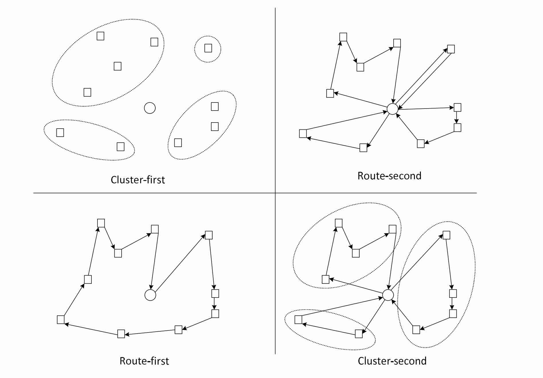
Figure from this presentation on clustering approaches.
While the first approach is more intuitive, the second can lead to a more efficient search in practice. A production system would use something in between these two options; it would build a route across the graph then use it as a loose suggestion to start creating clusters. Once we have clusters, we need to decide how individual packages will be delivered within a cluster.
Step 2: Ordering
Now that we have packages divided into clusters, we need to figure out:
- How to visit packages in each cluster.
- How to order the clusters to minimize redundant driving.
Problem 1 is essentially a TSP problem, with the added complexity that we have many options for where to start and finish each cluster. This impacts how a driver assigned multiple clusters might group them together. Since the package number in an individual cluster is small, we can just precompute a TSP for each start/finish combination using a variety of heuristics, and pick each cluster's start/finish to minimize the cost in Problem 2.
Problem 2 is actually a dynamic programming problem similar to edit distance, where we sequence clusters to minimize the total cost spent driving between clusters. However, once we figure out a decent arrangement of clusters, we destroy the clustering entirely and treat all of the packages as one route again. Then, we use iterated local search to explore newer routes that potentially cross cluster boundaries.
We can repeat this process of creating and destroying structure in the graph to escape local minima and find routes we're happy with. Our goal isn't to narrow the routes down to the best one, but rather to generate a lot of good potential routes which we will filter through in Step 4.
Step 3: Cost Analysis
A key step in optimizing our route generation algorithm is the ability to efficiently calculate the cost of a given route. When computing thousands or millions of TSP problems between nodes, we're doing an incredible amount of shortest-path queries, so it makes sense to start there.
Step 3.1: Shortest Paths
The classical algorithm for finding the shortest path between two nodes in a graph is Dijkstra's. It's got great theoretical performance, but there are many improvements we can make in a practical setting. This fantastic survey breaks down the major algorithms and how they perform on real road datasets, some of which include:
-
Goal-directed algorithms. While Dijkstra's computes
the shortest paths from a given source to all other nodes in the
graph, if we are only looking for a path between nodes (formally
called a "point-to-point query"), then we can
guide the algorithm to explore paths that get it closer to
the target node. The most famous goal-directed algorithm is
A* search,
frequently used for pathfinding in robotics and 3D games. Others
include
Geometric Containers, which takes
advantage of the graph being on a 2D map to
selectively look at paths that are geometrically feasible and
clustering, which precomputes distances between major clusters of
nodes to speed up a fresh computation.
-
Hierarchy-based algorithms. These take advantage of
the inherent hierarchy in a road network. For example, if we want to
find the shortest route between two towns, we might start with
taking local roads to get on a nearby highway, traveling close to
the target city, then switching to local roads again. Recognizing
that most routes follow a hierarchy of small road -> big road
-> small road is the basis for
Contraction Hierarchies,
which prioritizes routes which follow this model. Another choice
is
Reach, an algorithm which ranks how "central" each node is,
then first checks routes that go through central vertices (like how
most cities have a major highway interchange that lets you travel
basically anywhere.)
-
Bounded-hop algorithms. These are relatively new
compared to their counterparts, and involve precomputing shortest
paths between many nodes and using the precomputation as a
"virtual shortcut" during query time.
The shortest path problem on road networks is essentially a tradeoff between preprocessing time/space and query time.
Step 3.2: Auxiliary Factors
Transit time is far from the only cost associated with a route. Other factors include:
- How familiar a driver is with the route they are assigned to
- Whether a route violates an expected delivery time for a package
- Whether each driver gets a somewhat "balanced" route
These are considered by the routing logic in the form of penalties that are added to the cost of a route.
Step 4: Searching
After generating a few million potential routes for many different cluster configurations in Step 2, we need to mix and match them so that every package gets delivered exactly once. This becomes a set partitioning problem, which can be solved using integer linear programming as discussed in this presentation. The program's formulation is as follows:
There are many libraries that can provide an optimal solution in minutes, even on instances with 100K+ variables.
The context in which routes are created is also important; for example, the shortest path algorithms may need to preprocess in response to new traffic data. This is where insights from algorithm engineering are useful. The core problems in algorithm engineering concern how to run algorithms on large amounts of data that changes often, often by utilizing hardware acceleration or systems programming tools. A fair bit of background on the subject can be found in Julian Shun's graduate course.
Finally, a great way to tune the search parameters is by listening to direct feedback from delivery drivers. Drivers with years of experience in an area have intuition for what good routes are, and any serious company doing vehicle routing should use this intuition to improve their business logic. Even quick feedback like "how could your route have been planned better today?" can uncover issues quicker than test datasets or fuzzy testing.
Step 5: Delivery!
Hopefully, I've gone over a small fraction of the immense work it takes to get an Amazon package to my door in days (and in some cases, hours.)
The final step: packages in motion!