Efficiently Sampling Spanning Trees

Introduction

Sampling from complex distributions is at the heart of many problem-solving approaches in combinatorics and optimization. A common distribution is the set of all spanning trees on a connected graph, and a number of algorithms exist for constructing a uniform random sample efficiently. Some applications are:

Evaluating the reliability of networks by generating random routing patterns and stress-testing them
Sampling random Euler paths that have applications in genome sequencing and data analysis
Generating well-formed random mazes

Our goal is to walk through some helpful ideas and algorithms.

Random Edge-Weight MST

A project for University of Washington CSE 373 (Data Structures and Algorithms) asks students to generate a maze by the following method:

Create "rooms" and "walls" on a grid.
Assign each room to a vertex and each line (i.e. the border between two rooms) to an edge.
Assign each edge a random weight and run a minimum spanning tree algorithm.

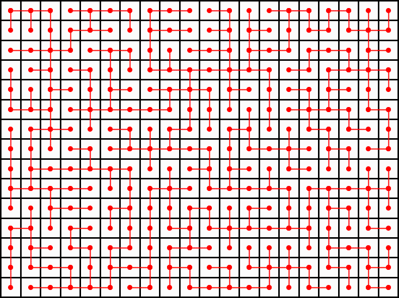
The resulting minimum spanning tree can be converted into a maze by deleting the walls corresponding to the edges that remain. This creates a well-formed maze because there is exactly one path from the top left corner to the bottom right, there are no unreachable rooms, and has an appropriate complexity due to its randomness. While this method is simple enough to be a coding exercise for a class project and produces visually appealing results, it is unfortunately not a uniformly random sample of all possible spanning trees of a graph. The following example illustrates why.

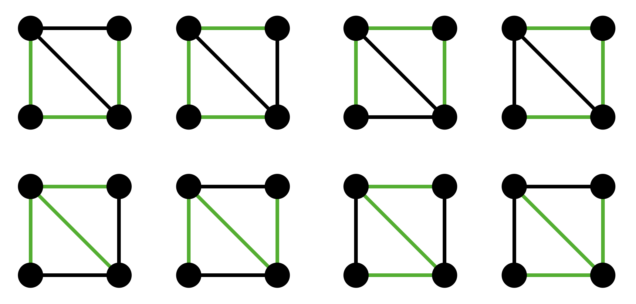
Suppose we have a graph with four vertices connected by five edges consisting of a square and diagonal. Then, the resulting graph has eight possible spanning trees, so we would expect that any one of them could be chosen with probability $1/8$. However, this is not true for the random edge-weight MST method.

Observe that there are four spanning trees that include the diagonal and four otherwise.

If we consider the random edge weights as creating a random permutation of the edges, then there are five equally likely cases for the diagonal edge:

The diagonal is first in the order (assigned the lowest weight randomly.) In this case, the diagonal is guaranteed to be included in the generated spanning tree.
The diagonal is second. In this case, the diagonal is still guaranteed to be included in the generated spanning tree.
The diagonal is third. Whether the diagonal is included in the spanning tree depends on the edge on the two edges that are before it. If it will create a cycle with the first two edges, then it will not be included. There are $\binom{4}{2} = 6$ different choices for the first two edges, and 2 of them result in the diagonal not being included. Thus, the probability that the diagonal is in the MST given that it is third in the random ordering is $2/3$.
The diagonal is fourth. It is guaranteed to not be in the MST.
The diagonal is fifth. it is not in the MST.

Since each of the cases is equally likely, we get that

$$\mathbb{P}(\text{diagonal in MST}) = \frac{1}{5} + \frac{1}{5} + \frac{2}{3} \cdot \frac{1}{5} = \frac{8}{15}$$

Even though half of the possible spanning trees contain a diagonal, the random edge-weight MST will pick a spanning tree with a diagonal more than half the time. While simple and intuitive, this method does not sample a uniformly random spanning tree. However, there is some work on how the resulting distribution behaves; [GS19] characterizes the separation between the random MST and the uniform distribution over trees as the number of vertices approaches infinity. The first paragraph of [A90b] states that the star graph is much more favored when sampling from $K_n$. While not truly random over all trees, this approach is useful in modeling fluid dynamics [DDMMDHM04] and remains an aesthetically pleasing way to generate a maze.

Prüfer Codes

We now formalize the problem and discuss methods to solve it. Let $G = (V, E)$ be an undirected connected graph with vertex set $V$ and edge set $E$. A spanning tree $S \subseteq E$ is a subset of the edges forming a tree that contains all vertices in $V$. Let $\mathcal{T}$ be the set of all spanning trees on $G$. Our goal is to create a random function $f: G \to S$ such that the probability of generating any given spanning tree is $1/|\mathcal{T}|$.

How large can $\mathcal{T}$ be? For $K_n$, the complete graph on $n$ vertices, Cayley [C89] calculates that $|\mathcal{T}| = n^{n-2}$. For any graph, we can calculate it using Kirchhoff's Matrix-Tree Theorem, which states that $|\mathcal{T}|$ can be computed by finding any cofactor of the graph's Laplacian matrix.

Theorem (Cayley's Formula)

For every $n > 0$, the number of trees on $n$ labeled vertices is $n^{n-2}$.

Theorem (Matrix-Tree Theorem)

For an undirected graph $G$ with spanning trees $\mathcal{T}$, $|\mathcal{T}| = \det L_G^{(ii)}$ for any $i$ where $L_G$ denotes the Laplacian of $G$ and $L_G^{(ii)}$ represents the $(i,i)$ minor of $L_G$.

We will prove the Cayley theorem repeatedly, and we defer the proof of the Matrix-Tree Theorem to later. These results prove that the number of possible spanning trees on a graph can be intractably large, which makes it computationally infeasible to generate the full set of spanning trees and pick one at random. Instead, we will aim to generate a sample stochastically, i.e. to construct a random process that samples from the space of all spanning trees with uniform probability without explicitly enumerating them all.

One such method is a Prüfer code. The philosophy of Prüfer codes is to encode each tree of $G$ into a unique sequence of numbers, then devise an algorithm to efficiently generate random encodings. An encoding is given by Prüfer [P18], who describes polynomial time procedures for encoding a tree on $n$ vertices as a sequence of $n-2$ vertices. At a high level, the sequence iteratively removes leaves and writes down their neighbors until two vertices remain.

Any sequence of $n-2$ integers in $\{1,2,\ldots,n\}$ is a Prüfer code for a unique tree on $n$ vertices. This directly gives a polynomial time algorithm for generating a random tree on $n$ vertices: assign each vertex a label, randomly generate $n-2$ integers, construct the tree. The decoding sequence naively takes $O(n^2)$ time, but we conjecture it is possible to optimize using combinations of arrays and linked lists. A glaring limitation of this method is that it samples a spanning tree on $K_n$ and cannot be restricted to a particular graph or edge set. We will turn our attention to specific graphs in the next section.

We can also use the uniqueness of Prüfer codes to prove Cayley's formula. There is a clear bijection between codes of size $n - 2$ and labeled trees on $n$ vertices. Since there are precisely $n^{n-2}$ such codes, we can conclude that the number of labeled trees on $n$ vertices is also $n^{n-2}$. □

Random Walks

While Prüfer codes are a straightforward technique to sample a uniform spanning tree on the complete graph $K_n$, they aren't helpful when we attempt to sample from a fixed undirected graph $G$. Thus we turn our attention to a much more powerful and theoretically popular technique: sampling a spanning tree via a random walk on $G$. This walk can be represented as a Markov chain, which unlocks the machinery used to study Markov chains and allows us to find efficient solutions to the spanning tree problem.

The basic algorithm is found in numerous notes and papers, but the simplest description of the walk is by Broder [B89]:

Simulate a simple random walk on $G$ starting at an arbitrary vertex $s$ until every vertex is visited. For each vertex $i \in V - s$ collect the edge $j, i$ that corresponds to the first entrance to vertex $i$. Let $T$ be this collection of edges.
Output the set $T$.

We will study the formulation given by Aldous in [A90a], discovered independently in the same year as Broder. Formally, let $G$ be an undirected connected graph on $n$ vertices. We define a random walk as a discrete Markov chain where each vertex is a state and the transition matrix $P$ is defined as

\[ P(u,v) = \begin{cases} 1/\text{deg($u$)} & \text{if $(u, v)$ is an edge} \\ 0 & \text{otherwise} \end{cases} \]

We begin a random walk on an arbitrary vertex $v_0$, denoted as $(v_0;\; j \ge 0)$. Then, for each vertex $u$ let $T_u$ be the first "hitting time" of $u$:

$$T_u = \min\{i \ge 0 : v_i = u\}$$

Then, we define our spanning tree to consist of the $n-1$ edges that "discover" a new vertex:

$$\mathcal{T}_G = \{(v_{T_v-1}, v_{T_v}) : v \neq v_0\}$$

The cover time $C$ of the walk is the time taken to visit all vertices:

$$C = \max_v T_v$$

It is clear why this walk produces a spanning tree — each vertex has an edge connected to it, and no cycles are created because that would require adding an edge between two vertices that have already been discovered, creating a contradiction. However, it is also true that this produces a uniform random spanning tree on $G$.

It is also clear that the running time of the algorithm is $C$. The walk is proven in [AKLR79] to have expected cover time $O(n^3)$, and for most graphs achieves $O(n \log n)$. These are due to connections between the structure of $G$ and the mixing time of the Markov chain, which are discussed briefly in [B89]. The Aldous, Broder, and similar formulations are treated as a family of random spanning tree algorithms called cover-time algorithms.

Proof of Aldous-Broder

We now prove that the Aldous-Broder algorithm produces a uniform spanning tree over $G$. Our strategy is:

Create a set $\mathcal{S}$ of rooted spanning trees on $G$.
Define a Markov Chain on $\mathcal{S}$ and connect it with the algorithm's walk.
Show that the chain on $\mathcal{S}$ has a uniform stationary distribution that is also its limiting distribution.
Extend to unrooted trees.

A rooted tree is a pair $(T, v)$ of a tree $T$ and a vertex $v$ in the tree that is considered the root of the tree. There are no modifications to the tree nor are we assigning directions to edges; this is simply defined for analysis. Let $\mathcal{S}$ be the set of all rooted spanning trees on $G$. Since every unrooted tree shows up exactly $n$ times in $\mathcal{S}$ with different roots, sampling uniformly from $\mathcal{S}$ is equivalent to sampling a random spanning tree.

We now define $S_i$ as the spanning tree generated by taking the random walk and only considering steps of the random walk at time $i$ and after:

$$T_u = \min\{j \ge i : v_j = u\}$$

We consider $S_i$ to be rooted at its first vertex, i.e. the vertex visited in the original walk at time $i$. Considering each $S_i$ a state, we see that the $S_i$'s form a Markov chain over $\mathcal{S}$. Then we consider the reverse transition probabilities $Q$ of $S_i$:

$$Q(t, t') = P(S_{-1} = t' \; | \; S_0 = t)$$

Let $\deg(t)$ be the degree of the root vertex of a tree $t$. Then we get two consequences:

Given $t$, there are exactly $\deg(t)$ trees $t'$ such that $Q(t, t') = 1/\deg(t)$, and $Q(t, t') = 0$ for all other trees $t'$.
Given $t'$, there are exactly $\deg(t')$ trees $t$ such that $Q(t, t') = 1/\deg(t)$, and $Q(t, t') = 0$ for all other trees $t$.

This means that for a fixed tree $t'$,

$$\sum_t \deg(t) Q(t,t') = \deg(t')$$

It can be shown that this implies the stationary distribution of the Markov chain on $\mathcal{S}$ is proportional to each tree's root degree $\deg(t)$. Furthermore, it is clear that this chain is irreducible as we can reach any $t$ from some other $t'$ by taking the path to the root vertex and constructing a depth-first search which leads to $t$.

Since the chain on $\mathcal{S}$ has stationary distribution equivalent to $\deg(t)$, and each unrooted spanning tree shows up with every vertex as a root exactly once, we can "marginalize" the root and we get that the algorithm samples each unrooted spanning tree uniformly. □

The use of "reverse transition probabilities" is a brief window into a long line of work analyzing reversible Markov chains and their applications to graph theory. The reader may survey Aldous' work for generalized results and another proof of Cayley's formula.

Wilson's Algorithm

It turns out that Aldous-Broder is the most straightforward of the walk-based algorithms but not the fastest. In fact, Wilson [W96] gives a result which is never slower than Aldous-Broder, and faster in many cases. Yuval Wigderson gives a nice formulation, which we restate. Given $G$ and a root vertex $r$, we define a growing sequence of rooted trees $T_i$ as follows:

Set $T_0$ to be $r$.
If $T_i$ is a spanning tree on $G$, stop and output. Otherwise, pick a random vertex $v$ not in $T_i$ and run a random walk from $v$ until a vertex in $T_i$ is hit. Erase loops in the path from $v$ to $T_i$, then set $T_{i+1} = T_i \cup v$.

This algorithm works for weighted or directed graphs as well, and produces the analog of a uniform random spanning tree in those settings. We skip the proof, but note that the running time is improved from the cover time to the mean hitting time of the graph.

Unexplored Directions

An alternate method similar to Prüfer codes is given in [CDN89]. The authors assign each spanning tree a ranking within the set of all spanning trees, then describe an $O(n^3)$ algorithm for converting between a rank and a spanning tree on $G$. Counting the number possible spanning trees then generating a random rank yields an $O(n^3)$ method for sampling from spanning trees.
It can also be observed that spanning trees form the bases of a matroid on $G$, and thus we can use machinery created to sample from bases of a matroid to achieve the goal. There is active work at the University of Washington being done in this area; the reader may survey [S22] and its listed references if interested.
The proof of Cayley's/Matrix-Tree result hinges on the fact that for any edge $e$, if $G-e$ is the graph without $e$ and $G \cdot e$ is the graph with $e$ contracted, the number of spanning trees on $G$ is the sum of the trees on $G-e$ and $G \cdot e$. This implies a simple algorithm by Guénoche in [G83] that repeatedly deletes and contracts edges until a spanning tree is created. It can been shown that this algorithm runs in $O(n^5)$.

Deferred Proof of Kirchhoff's Theorem

We prove the Matrix-Tree Theorem by induction, restating the proof given by Moore (see [M11]). The base case is a graph with a single vertex and no edges. The minor of its Laplacian will be the $0 \times 0$ matrix, which has determinant 1, so the result holds. Assume that the result holds for graphs with fewer vertices or edges. For the inductive step, choose a vertex $i$ and suppose that $G$ has two or more vertices. If $i$ has no edges, $G$ is disconnected and no spanning trees exist; the determinant of the Laplacian will be zero. So we can assume that $i$ is connected to another vertex $j$ via an edge $(i,j)$ which we call $e$.

We consider two modifications to $G$: deleting $e$ to make $G-e$, and contracting the edge to merge $i$ and $j$ into a single vertex, making $G \cdot e$. We observe (skipping a proof) that the number of spanning trees on $G$ is the sum of the trees on $G-e$ and $G \cdot e$. Now reorder the vertices of $G$ such that $i$ and $j$ are the first two, and we can write the Laplacian of $G$ as the following:

$$ L_G = \left( \begin{array}{c|c|c} d_i & -1 & r_i^T \\ \hline -1 & d_j & r_j^T \\ \hline r_i & r_j & L' \end{array} \right) $$

Here $r_i$ and $r_j$ are $(n-2)$-dimensional column vectors describing the connections between $i$ and $j$ and the other $n-2$ vertices, and $L'$ is the $(n-2)$-dimensional minor describing the rest of the graph. We can write the Laplacians of $G-e$ and $G \cdot e$ as

$$ L_{G-e} = \left( \begin{array}{c|c|c} d_i - 1 & 0 & r_i^T \\ \hline 0 & d_j - 1 & r_j^T \\ \hline r_i & r_j & L' \end{array} \right), \quad L_{G \cdot e} = \left( \begin{array}{c|c} d_i + d_j - 2 & r_i^T + r_j^T \\ \hline r_i + r_j & L' \end{array} \right) $$

To finish the induction, we want to show that

$$\det L_G^{(ii)} = \det L_{G-e}^{(ii)} + \det L_{G \cdot e}^{(jj)}$$

which corresponds to

$$\det \left(\begin{array}{c|c} d_j & r_j^T \\ \hline r_j & L' \end{array}\right) = \det \left(\begin{array}{c|c} d_j - 1 & r_j^T \\ \hline r_j & L' \end{array}\right) + \det L'$$

But this follows from the fact that the determinant of a matrix can be written as a linear combination of its cofactors, i.e., the determinants of its minors. Specifically, for any $A$ we have

$$\det A = \sum_{j=1}^{n} (-1)^j A_{1,j} \det A^{(1,j)}$$

Thus if two matrices differ only in their $(1,1)$ entry, with $A_{1,1} = B_{1,1} + 1$ and $A_{ij} = B_{ij}$ for all other $i,j$, their determinants differ by the determinant of their $(1,1)$ minor, $\det A = \det B + \det A^{(1,1)}$. Applying this to $L_G^{(ii)}$ and $L_{G-e}^{(ii)}$ yields the above equation and completes the proof. □

This result is often used to prove Cayley's formula. The Laplacian of $K_n$ looks like:

$$ \begin{bmatrix} n-1 & -1 & \cdots & -1 \\ -1 & n-1 & \cdots & -1 \\ \vdots & \vdots & \ddots & \vdots \\ -1 & -1 & \cdots & n-1 \end{bmatrix} $$

which has determinant $n^{n-2}$ for any $(i,i)$-minor.

A PDF version of these notes is available here.

References

[GS19] Christina Goldschmidt. Random minimum spanning trees. Mathematical Institute, University of Oxford, 2019. Retrieved 2019-09-13.
[A90b] David J. Aldous. A Random Tree Model Associated with Random Graphs. Random Structures and Algorithms, 1(4):383–402, 1990. doi:10.1002/RSA.3240010402.
[DDMMDHM04] P. M. Duxbury, R. Dobrin, E. McGarrity, J. H. Meinke, A. Donev, C. Musolff, and E. A. Holm. Network Algorithms and Critical Manifolds in Disordered Systems. In David P. Landau, Steven P. Lewis, and Heinz-Bernd Schüttler, editors, Computer Simulation Studies in Condensed-Matter Physics XVI, pages 181–194, Berlin, Heidelberg, 2004. Springer Berlin Heidelberg.
[C89] A. Cayley. A theorem on trees. Quarterly Journal of Pure and Applied Mathematics, 23:376–378, 1889.
[P18] Heinz Prüfer. Neuer Beweis eines Satzes über Permutationen. Archiv der Mathematik und Physik, 27:742–744, 1918.
[B89] A. Broder. Generating random spanning trees. In Proc. 30'th IEEE Symp. Found. Comp. Sci., pages 442–447, 1989.
[A90a] David J. Aldous. The Random Walk Construction of Uniform Spanning Trees and Uniform Labelled Trees. SIAM Journal on Discrete Mathematics, 3(4):450–465, 1990. doi:10.1137/0403039.
[AKLR79] R. Aleliunas, R. M. Karp, R. J. Lipton, L. Lovász, and C. Rackoff. Random walks, universal traversal sequences, and the complexity of maze traversal. In Proc. 20th IEEE Symp. Found. Comp. Sci., pages 218–233, 1979.
[W96] David Bruce Wilson. Generating random spanning trees more quickly than the cover time. In Proceedings of the Twenty-Eighth Annual ACM Symposium on Theory of Computing, STOC '96, pages 296–303, New York, NY, USA, 1996. Association for Computing Machinery. doi:10.1145/237814.237880.
[CDN89] Charles J. Colbourn, Robert P.J. Day, and Louis D. Nel. Unranking and ranking spanning trees of a graph. Journal of Algorithms, 10(2):271–286, June 1989. doi:10.1016/0196-6774(89)90016-3.
[S22] Tselil Schramm. Lecture 5: Approximate Sampling of Spanning Trees via Matroid Basis Exchange. Lecture notes for STATS 221: Random Processes on Graphs and Lattices, Stanford University, January 19, 2022. Available at https://web.stanford.edu/class/stats221/.
[G83] A. Genoche. Random Spanning Tree. J. Algorithms, 4:214–220, 1983.
[M11] Cristopher Moore. The nature of computation. Oxford University Press, Oxford, England New York, 2011. ISBN 978-0-19-923321-2.